Basic Uses of Cursor

esProc supports importing big data in batches with the cursor, which is the usual method for big data computing. Different types of cursors, including database cursor, external file cursor and in-memory record sequence cursor, basically work the same way. This part takes the external file cursor as the example to explain basic uses of the cursor in esProc.

7.2.1 Data fetching

When a cursor is created, its data can be fetched with cs.fecth() function. Different from an ordinary table, usually data in the cursor won’t be fetched all at once; it is fetched instead by specifying the number of rows to be returned, or one or more data fetching conditions. For example:

	A
1	=file("Order_Books.txt")
2	=A1.cursor@t()
3	=A2.fetch(1000)
4	>A2.close()
5	=A2.fetch(1000)

A2 creates an external file cursor. A3 fetches the first 1,000 rows from it:

With fetch function, each batch of data fetched from the cursor will be returned as a table sequence. A4 calls cs.close() function to close the cursor. When a cursor is closed, data cannot be fetched from it. That is why the result of A5 is null:

When a cursor has accomplished its mission and won’t be needed any more, it ought to be closed through calling cs.close() function to release the memory.

Besides fetching data from the file or the database result set through the cursor, a specified number of rows in the cursor can be skipped using cs.skip() function. For example:

	A
1	=file("Order_Books.txt")
2	=A1.cursor@t()
3	>A2.skip(45000)
4	=A2.fetch()
5	=A2.fetch(1000)

A2 creates a cursor and A3 skips 45,000 rows. Then A4 fetches data from the cursor:

According to the transaction IDs, the data fetching begins from the 45001th row. Notice that the fetch function in A4 doesn’t specify the number of rows to be returned. In this case, all the rest of the data in the cursor will be fetched. Once data in the cursor is completely fetched, the cursor will close automatically, without the necessity of calling cs.close() function.

So A5 fetches nothing from A2’s cursor:

In fact, both cs.skip() function and cs.fecth() function will traverse the cursor data once in a forward-only fashion. When the data fetching is over or cs.close() function is executed, the cursor becomes useless.

Another type of fetching data from the cursor using cs.fecth() function is cs.fetch(;x), which specifies the condition according to which data fetching will continue uninterruptedly until the value of expression x changes. For example:

	A
1	=file("Order_Books.txt")
2	=A1.cursor@t()
3	=A2.fetch(;Date)
4	=A2.fetch(1000)
5	>A2.close()

A2 creates a cursor. A3 fetches data from it until the value of Date changes. The fetched data is as follows:

A3 fetches all data whose Date value is 2013-01-01. When A4 goes on with fetching data from A2’s cursor, it will begin from the date 2013-01-02:

Note that you shouldn’t specify both the number of rows to be returned and data fetching condition at the same time; otherwise only the latter is valid. Besides, since not all the data in A2’s cursor has been fetched, the cursor needs to be closed in A5 after doing its job.

Similarly, a condition can also be specified in cs.skip() function to skip certain records:

	A
1	=file("Order_Books.txt")
2	=A1.cursor@t()
3	>A2.skip(;Date)
4	>A2.skip(;Date)
5	>A2.skip(;Date)
6	=A2.fetch(1000)
7	>A2.close()

A2 creates a cursor. A3, A4 and A5 respectively skip records of one day. Then A6 fetches data from the cursor from the fourth day:

Similarly, if not all the data has been fetched from the cursor, call cs.close() function in A7 to close the cursor.

7.2.2 Cursor loop

for statement can be used to fetch data from a cursor by loop. For example:

	A	B
1	=file("Order_Books.txt")
2	=A1.cursor@t()	0
3	for A2,1000	=A3.select(SalesID==1).sum(Amount)
4		>B2=B2+B3

A2 creates a cursor. A3 loops through records of the cursor to fetch 1000 records each time. After all records are traversed, the cursor will close automatically. A3’s code block computes the total sales amount of the salesperson whose ID number is 1 and stores the result in B2 based on each table sequence returned by the cursor. Here’s the final result:

But sometimes not all records need to be traversed for a cursor loop. For example:

	A	B	C
1	=file("Order_Books.txt")
2	=A1.cursor@t()	[]
3	for A2,1000	=A3.select(SalesID==1)	>B2=B2|B3
4		if B2.len()>=5	>B2=B2(to(5))
5			break
6	>A2.close()

A2 creates a cursor and A3 executes a cursor loop, fetching 1,000 records each time. A3’s code block selects the sale records of the salesperson whose ID number is 1 and stores them in B2 according to each batch of data fetched from the cursor. Exit the loop after the first 5 records are fetched. At this point the result in B2 is as follows:

One point worthy of special note: When the computation is over and the loop is terminated by break function, there is still data in the cursor, which is different from the previous example. So the cursor won’t close automatically, and close function is called in A6 to close it and release the memory.

Similar to cs.fetch() and cs.skip(), a condition can be specified for a cursor loop so that the data fetching will stop as soon as the value of the conditional expression changes. For example:

	A	B	C
1	=file("Order_Books.txt")
2	=A1.cursor@t()	=create(Date,Count,Amount)
3	for A2;Date	=A3.count()	=round(A3.sum(Amount))
4		>B2.insert(0,A3.Date,B3,C3)

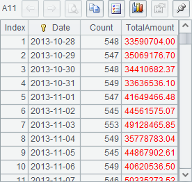
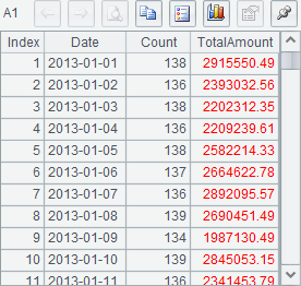
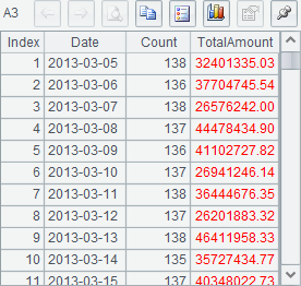
With the condition, A3 fetches the sales data of one day each time, computes the number of transactions and the total sales amount in this day in its code block and stores the results in B2’s table sequence. After the code is executed, B2’s table sequence is as follows:

7.2.3 Cursor-based operations

Besides fetching data from a cursor, esProc also offers performing common data computations by directly using certain functions. The following example is a conditonal query based on the cursor:

	A	B
1	=file("Order_Books.txt")	=A1.cursor@t()
2	=B1.select(SalesID==1)	=A2.fetch()
3	=A2.fetch()	=B1.fetch()

B1 creates an external file cursor and A2 selects the sales data of the salesperson whose ID number is 1 from B1’s cursor. Here’s A2’s result:

You can see that A2 and B1 get the same result. Different from the select function with a table sequence or a record sequence, the select function used with a cursor returns the cursor itself. A2’s operation doesn’t really get data from the cursor. It is actually a bundled operation. It is in B2 where cs.fecth() function is being executed that the data queried and fetched from B1’s cursor according to the condition. Here’s B2’s result:

No number of rows to be returned or a data fetching condition is specified for cs.fetch() function used in B2. Thus all data in A2’s cursor, i.e. all the sales data of the specified salesperson, will be returned, and the cursor will close automatically. The cursor in A2 is equivalent to the one in B1, and actually during the data query, it is B1’s cursor data that is traversed during which the bundled data fetching is executed. So as the data in A2’s cursor is fetched out, B1’s cursor will be fetched out too, and close. Therefore the effort of A3 and B3 trying to fetch data from the cursors in both A2 and B1 will definitely fail.

If the data in a file is already sorted, you can use f.iselect(A,x,Fi,…;s) or f.iselect(a:b, x,Fi,…;s) to select data to generate cursor, which is more efficient. For example:

	A	B
1	=file("Order_Books.txt").iselect@t(["S020000012", "S020000022"],ID; ID,PID,Date,Amount)	=A1.fetch()
2	=file("Order_Books.txt").iselect@ti(date(2013,2,1): date(2013,2,28),Date; ID,PID,Date,Amount)	=A2.fetch@x(100)

Since the file contains field names, @t option is used. Similarly, if it is a bin file, @b option can be added. A1 uses f.iselect(A,x,Fi,…;s) to get the sales records by order ID. By default iselect function requires the desired data is distinct when performing a search. A2 searches for sales records during a specified time period using f.iselect(a:b, x,Fi,…;s) function with an @i option, meaning there could be more than one Date and all eligible records will be returned. When executed, B1 and B2 get results as follows:

You can also create new records or append new fields based on a cursor. For example:

	A	B
1	=file("employee.txt")	=A1.cursor@t(EID, NAME,SURNAME, GENDER, STATE,BIRTHDAY)
2	=B1.new(EID, NAME+" "+SURNAME:FullName, GENDER,STATE,BIRTHDAY)	=B1.derive(age(BIRTHDAY):Age)
3	=A2.fetch(100)	=B2.fetch(100)
4	>A2.close()	=B2.fetch()
5	>B2.close()

B1 creates a file cursor using some of the fields of the external file employee.txt. A2 generates employees’ full names by joining NAME field and SURNAME field in B1’s cursor. B2 computes each employee’s age according to the BIRTHDAY field in B1’s cursor and enter the results to Age field. Similar to cs.select(), both cs.new() and cs.derive() return a cursor, rather than returning data directly. When executed, A2 and B2’s cursor values are the same as B1’s:

Here are the first 100 rows fetched from A3:

Generating data with cs.new() function means executing new statement on every record.

Here are the first 100 rows fetched from B3:

Generating data with cs.derive() function means appending computed columns to the returned table sequence.

B3’s data has the same structure as A3’s data. It begins from the 101th employee. That’s because both A2 and B2 have a bundled operation with their cursors while both fetch data from the same cursor, and a cursor will be traversed only once in a forward direction. After A3 is executed, the first 100 rows have been traversed. So B3 can only continue the traversal in order by beginning with the 101th employee when executing the cs.fecth() function.

But as data hasn’t been all fetched out in both cursors, they need to be closed using cs.close() function. As A4 closes the cursor in A2, the cursor in B1 is also closed simultaneously, for A2 and B1 are in reality the same cursor. A try of fetching more data thus fails.

What’s more, cs.run() function can be used to modify values of a certain field in cursor:

	A	B
1	=file("employee.txt")	=A1.cursor@t(EID, NAME,SURNAME, GENDER, STATE,BIRTHDAY)
2	=demo.query("select STATEID, NAME, ABBR from STATES")	=B1.run((a=STATE,STATE=A2.select@1(NAME==a).ABBR))
3	=B2.fetch(100)	>B2.close()

B2 replaces names of the states in the returned data with their abbreviations and returns a cursor with a bundled operation:

A3 fetches the first 100 rows:

Similar to a table sequence, the cursor allows the switch between one of its fields and the corresponding records in another table sequence by using cs.switch() function. For example:

	A	B
1	=file("employee.txt")	=A1.cursor@t(EID, NAME,SURNAME, GENDER, STATE,BIRTHDAY)
2	=demo.query("select STATEID, NAME, ABBR from STATES").keys(STATEID)	=B1.switch(STATE,A2:NAME)
3	=B2.fetch(100)	>B2.close()

B2 uses cs.switch() to convert certain data of the cursor. The result is still a cursor with a bundled operation:

Here’s the result of data fetching in A3:

In the result values of STATE field have been converted into the corresponding state records.

The cs.switch() function can convert more than one field of the cursor. For example:

	A	B
1	=file("employee.txt")	=A1.cursor@t(EID, NAME,SURNAME, GENDER, STATE,BIRTHDAY)
2	[F,Female,M,Male]	=create(ID,Gender).record(A2).keys(ID)
3	=demo.query("select STATEID, NAME, ABBR from STATES").keys(STATEID)	=B1.switch(GENDER,B2;STATE,A3:NAME)
4	=B3.fetch(100)	>B3.close()

B3 switches values of several fields of the cursor to the corresponding records in another table sequence. A4 fetches the first 100 records:

Primary Key and Index explained the use of switch function in the ordinary table sequences, which is similar to that of cs.switch() in external memory computations. Both functions will create the index table for certain field(s) of the dimension table in order to increase efficiency. It is more important to adopt this processing method while using the cursor because usually the data under processing is big.