Simple SQL

The functionalities explained in the following content only appear in the esProc Enterprise Edition, users who use the other editions just skip it.

This section illustrates the basic uses of simple SQL and how they work with esProc ODBC.

9.4.1 Basic uses

esProc supports querying TXT and CSV files directly. It uses the SQL-like database statements to do that. We call it simple SQL, and the TXT and CSV files, which are external data that is queryable as table sequences, the external tables. For example:

	A
1	$()select * from cities.txt
2	$select * from D:/files/txt/cities.txt where STATEID=5
3	$select STATEID, count(*) AS Cities from cities.txt group by STATEID

Similar to a database SQL query with data source connected, esProc writes the simple SQL statement directly after the dollar sign ($) to query data from an external table. If a database connection exists, the statement after $ will by default executed in the database. To use simple SQL to query data in an external file, we can add () after the dollar sign $. Below is A1’s result set of querying cities.txt:

The simple SQL statement in A1 directly uses the file name instead of a specific table name. That’s the difference from a SQL statement. The file should be in esProc’s main path if the file path isn’t explicitly written. In the query, the type of file used is determined by its extension. A simple SQL statement supports using text files with txt or csv extension, Excel files with xls or xlsx extension, and bin files with the btx extension.

You can set a filtering condition where or calculate aggregate in a simple SQL statement. For example, A2 gets city records where STATEID is 5; and A3 counts the cities in each group of state records. Below are their result sets:

Similar to the usual SQL syntax, an aggregate function performing the corresponding aggregate operation needs to work with the group by clause that performs the grouping operation. Besides the count aggregation function, we can use sum/max/min/distinct function in a simple SQL statement.

The file name of an external table in a simple SQL statement can be represented by a full path, like the one A2 uses.

Query data in an external table and return part of the data:

	A
1	$select top 5 CID, NAME, POPULATION from cities.txt
2	$select CID, NAME, POPULATION from cities.txt limit 2 offset 3
3	$select * from cities.txt where STATEID < 20 and POPULATION<300000

A1 retrieves the first n records using top n:

A2 performs page skipping query using limit n offset m, which skips the first m records to retrieve n records. Below is the result:

Actually, a where filtering operation can also return part of data. Like the SQL rule, connect multiple filtering conditions, if there are any, with and. Logical operators, such as or/not, can also be used as needed. Below is A3’s result:

 

In a simple SQL statement, we can specify an alias for a table or field to be queried. For example:

	A
1	$select CID as ID, NAME as CITY, POPULATION as POP from cities.txt
2	$select CID ID, NAME CITY, POPULATION POP from cities.txt
3	$select distinct _file, _ext, _size, _date from cities.txt
4	=A3.derive(datetime(_date):date)

Like the SQL syntax, SPL can use keyword as to set an alias or just omit it. A1 and A2 return the same result, as shown below:

In addition to fields of a data table, the simple SQL can be used to query file information. _file, _ext, _size and _date respectively return a file’s name, extension, size and the last modified time, and keyword distinct removes duplicate information. A3 gets the following result:

A4 converts the last modified time to a date type time and gets the following result:

In a simple SQL statement, we can use a subclause, such as join/left join/right join/full join, to connect multiple tables to perform a multi-table query. For example:

	A
1	$()select * from states.txt
2	$select C.CID as ID, C.NAME as City, C.POPULATION as Pop, S.NAME as STATE  from cities.txt C join states.txt S on C.STATEID = S.STATEID
3	$select C.CID as ID, C.NAME as City, C.POPULATION as Pop, S.NAME as STATE  from cities.txt C full join states.txt S on C.STATEID = S.STATEID
4	$()select C.CID as ID, C.NAME as City, C.POPULATION as Pop, S.NAME as STATE  from cities.txt C left join states.txt S on C.STATEID = S.STATEID

Check A1’s result set and we can see that states.txt stores some state information:

A2, A3 and A4 perform join queries – inner join, full join and left join respectively, on cities table and states table, and get the following results:

 

When performing a grouping operation, we can use group by n to specify the nth field or expression used in the select statement as the grouping field/expression. For example:

	A
1	$select STATEID, count(*) Cities from cities.txt group by STATEID
2	$select STATEID, count(*) Cities from cities.txt group by 1
3	$select STATEID, count(*) Cities from cities.txt group by STATEID having Cities > 1
4	$select STATEID, count(*) Cities from cities.txt group by STATEID having Cities > 1 order by Cities

A2 gets the same result as A1:

A3 uses having clause to perform a filtering during the grouping operation and returns the following result:

A4 uses order by clause to sort the result set after A4’s grouping and filtering operations, and get the following result:

As the syntax group by n, we can write order by clause as order by n to sort records, where n is the ordinal number of a field in the select statement.

 

We can use wildcard characters in a simple SQL statement to query desired data from multiple external files having similar names and same structure. For example:

	A
1	$(demo) select * from STATES where STATEID<5
2	$select * from STATES where STATEID>10 and STATEID<15
3	$()select * into statePart1.txt from {A1}
4	$select * into statePart2.txt from {A2}
5	$select * from statePart*.txt

A1 and A2 respectively query certain states information from database demo, and get the following results:

A3 and A4 use select… into subclause to store A1’s data and A2’s data to external files statePart1.txt and statePart2.txt respectively, and determine file types according to file extensions. Since the previous query is a database one, A3 needs to begin the simple SQL statement querying an external file with $(). In the simple SQL statement, an esProc expression referenced should be enclosed by {}. To call A1’s result table sequence using {A1}, for example:

A5 performs wildcard matching to retrieve records from data files whose names match statePart*.txt, and concatenate them. Here these files must have the same structure. Below is A5’s result:

9.4.2 Using simple SQL in esProc ODBC

You can choose to skip this section if you are not a professional programmer. This won’t affect your learning about the other contents of this Tutorial.

esProc ODBC supports external data sources that are data files with the commonly seen formats like txt, csv, xls and xlsx, that are esProc bin files, which are discussed in detail in Bin Files, and that the base table of a composite table, which is expounded in Generating a composite table.

You can also use a simple SQL statement in esProc ODBC to query an external table. For example:

	A
1	=esProcOdbc.query("select PName, SalesID, Date from Order_Electronics.txt where Amount>200000 and month(Date)=5")
2	$(esProcOdbc) select Date, count(ID) as Count, sum(Quantity) as Sum from Order_Electronics.txt group by Date
3	$(esProcOdbc) select Date, count(ID) as Count, sum(Quantity) as Sum from Order_Electronics.txt group by 1
4	$(esProcOdbc) select Date, count(ID) Count, sum(Quantity) Sum from Order_Electronics.txt group by Date having sum(Quantity)>110000 order by Sum

To make a txt file an external table, use tab as the column separator.

A1 uses where to specify a query condition in the simple SQL statement to get the orders data where the sales in May are greater than 200,000. Here’s the result:

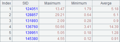
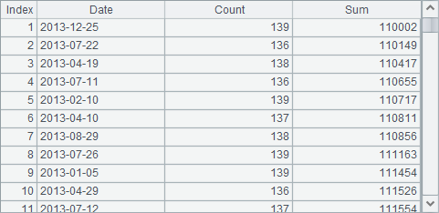
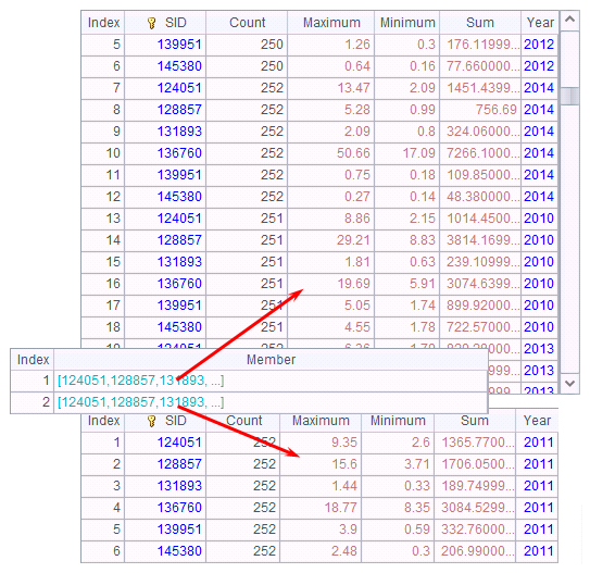
The simple SQL statement in A2 groups data by Date using the group by clause and calculates the number of orders per day and the quantity of products sold per day using the aggregate functions count and sum, while naming certain fields in the result set with as. You can also use other aggregate function like max/min/distinct in a simple SQL statement. Here’s the result set in A2:

In A3’s simple SQL statement, instead of a field name, the group by is followed by ordinal number 1, which means grouping data by the first expression in the select part. This will get the same result as A2.

A4’ query uses the having clause after group by to get records where the sum(Quantity) value is greater than 110,000 from the result set, omits as and uses the order by clause at the end to sort the result set by Sum in ascending order. Here’s the query result:

A simple SQL statement can join two external tables. For example:

	A
1	$(esProcOdbc) select StateId, Name, Abbr from states.txt
2	$(esProcOdbc) select NAME,POPULATION,STATEID from cities.txt
3	$(esProcOdbc) select C.NAME,C.POPULATION, S.StateId, S.Abbr from states.txt S join cities.txt C on S.StateId=C.STATEID
4	$(esProcOdbc) select C.NAME,C.POPULATION, S.StateId, S.Abbr from states.txt S left join cities.txt C on S.StateId=C.STATEID

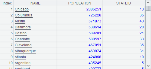
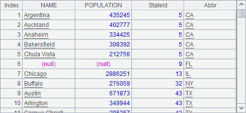
A1 and A2 retrieve data from states.txt and cities.txt. Their results are as follows

A3 joins the two external tables to get records of cities whose states abbreviations can be found. Here’s the result:

A4 uses a left join to get the following result:

An external table can be defined by a with, as shown in the following code:

	A
1	$(esProcOdbc) with C as (select*from cities.txt), S as (select * from states.txt) select C.NAME,C.POPULATION, S.StateID, S.Abbr from S join C on S.StateID=C.STATEID
2	$(esProcOdbc) with C as (select * from cities.txt), S as (select * from states.txt), select C.NAME Name,C.POPULATION Population, S.StateID StateID, S.Abbr Abbr into citiesInfo.btx from S join C on S.StateID=C.STATEID
3	$(esProcOdbc) select * from citiesInfo.btx

The query result in A1 is the same as that in A3 in the previous cellset.

A2 uses select…into T… statement to store the query result in another external table T. You can retrieve the data from the external table T after the store is complete