Properties of general cells
This section illustrates Value, Layout, Paragraph, Font, Expansion, Hyperlink, Page Break and Other properties for general cells.
Value
This section involves property value, display format and display value of a general cell.
Value
The first item in the cell property list is “Value”. The value refers to the cell’s actual value. When a cell is referenced, it is its actual value that is referenced.
● Example: Result of computing expression A1+B1 is value of cell A1 plus that of cell B1.
Display Format
The “Display Format” is the second item of the cell properties list. It is used to set the format of displaying a value in a report.
● Example:
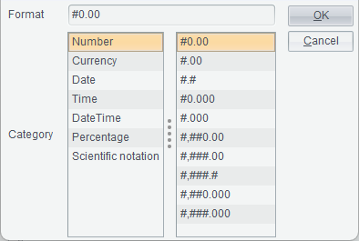
If value of a cell is a numeric data, like 1.33333, and we expect to round it up and display a decimal with two decimal places. The process is achieved through configuring the display format. You can edit #0.00 for the display format property value and a preview shows that the display number becomes 1.33.
You can also double-click “Display Format” property and get the following “Formatting” dialog box to select a right format and click “OK”, as the following screenshot shows:
Display Value
The third item in the cell properties list is “Display Value”. A display value is the content to be displayed in a report. It is only used for display, and seldom for reference. If you need to reference the display value of a cell, use disp function, such as disp(A1), which represents A1’s display value.
Generally, A field value retrieved from a data table is a symbol. But that isn’t what we expect to display in a report. We hope to display the actual value the symbol represents, and use display value property to achieve this.
There are two types of display value definition – “single value” and “reference table”.
● Example:
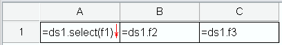
By single value:
1. "China", for instance, and the cell value is displayed as "China".
2. ds1.select(name,id == value()), for instance; according to the expression, we find the id equivalent to the current cell value from data set ds1, and according to this id, display corresponding name field value.
By reference table:
map(list(0,1),list("Male","Female")); if the cell value is 0, the cell displays Male in the report; and if the cell value is 1, the cells displays Female in the report.
Layout
This section illustrates visible, hidden row, hidden column, forecolor, backcolor, resize mode properties of general cells.
Visible
Choose whether the current cell is visible or invisible. A cell is visible when setting true as the property value, and invisible when setting false as the property value. You can control the “Visible” property in row primary cell, column primary cell, general cells or report primary cell.
The property can be represented by a value or an expression. In many occasions, we need to specify that the property is displayed when a certain condition is met and won’t be displayed when the condition isn’t met. To achieve this, we can edit a conditional expression for the property.
●Example expression:
if(@arg1=="raqsoft",true,false) When parameter arg1’s value is raqsoft, the current cell is visible, otherwise it is invisible.
Hidden Row
Choose whether to hide the current row. The property can be represented by a value or an expression.
To hide the current row, you can click “Hidden Row” property or select “Visible” property in row primary cell’s row properties.
If you set up the “Visible” property for the row primary cell, the configured property will be copied to “Hidden Rrow” property of all cells in the row.
● Example:
Edit =to(1,10) in A1. If you want to hide the corresponding row when value of the current cell is 5, edit if(A1==5,true,false) for “Hidden Row” property, or “Visible” property of row properties of the row primary cell. The preview shows that the row is hidden when A1’s value is 5.
If you want to hide a row whenever any cell in this row has a negative value, edit expression if(value()<0,true,false) for “Hidden Row” property of the row’s primary cell. This property expression will be copied to all cells expanded from this row.
Note: Hidden rows are not allowed for a report with clustered columns.
Hidden Column
Choose whether to hide the current column. The property can be represented by a value or an expression.
You can hide the current column through configuring the related property of a general cell or a column primary cell. See “Hidden Row” property to learn about when to configure a general an when to configure a column primary cell.
ForeColor
Set the color of text in a cell.
● Example: As the following shows (the left is the default foreground color <black>, and the right is the configured red color).
![]()
Note: Excel supports 256 colors only, but ReportLite supports any colors. So, certain colors do not have counterparts when being exported to Excel. In that case, the system will find the nearest Excel color.
BackColor
Set background color of a cell.
● Example: As the following shows (the left is the default foreground color <white>, and the right is the configured red color).
![]()
Note: Excel supports 256 colors only, but ReportLite supports any colors. So, certain colors do not have counterparts when being exported to Excel. In that case, the system will find the nearest Excel color.
Resize Mode
There are four options – “Fixed”, “Resize according to content”, “Fill up cell with image” and “Reduce font size to fill”.
1. By selecting “Fixed”, data will be displayed according to the current width of the cell when content is out-of-bounds.
2. By selecting “Resize according to content”, width of a cell will automatically change according to the content when data is out-of-bounds. For a cell holding a subreport or an image, you can choose to zoom out the subreport or the image to fit the cell or stretch out the cell to fit the content.
3. By selecting “Fill up cell with image”, the image will be zoomed in or out according to the size of the cell to ensure that the image is able to fill up the cell.
4. You can select “Reduce font size to fill” when content of a cell is exceeds the current cell width and when you do not want to stretch out the cell. By selecting this option, font size will reduce to fit the cell. If “Auto-wrap Text” is selected at the same time, data in the cell, besides the smaller font size, will be wrapped and displayed in multiple lines. Cooperation of the two options helps to avoid too small font size in order to display data in a cell in just a single line.
Paragraph
This section explains auto-wrap text, alignment mode and indentation in details.
Auto-wrap Text
You can choose whether to automatically wrap a line when the data length of the current cell exceeds the cell width.
This property usually applies to Chinese field values. Once it is checked, text will be automatically wrapped into a new line and the cell will automatically become higher when data length exceeds width of the cell.
For instance, when both “Auto-wrap Text” and “Reduce font size to fill” are selected for a cell, content will be wrapped and font size reduced for very long text and the system will automatically select the optimal algorithm according to the size of the cell.
● Example: Cell C3 contains a string as follows:
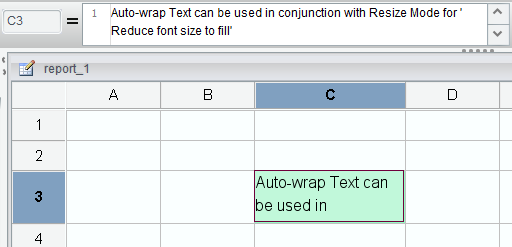
When “Auto-wrap Text” is selected, the preview effect is:
The cell becomes higher and the text is wrapped to be displayed in multiple lines.
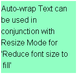
when both “Auto-wrap Text” and “Reduce font size to fill” are selected, you get the following preview effect:
The width and height of the cell do not change, but the text is displayed in smaller font size in multiple lines.
● Note:
For a report, “Auto-wrap Text” property only applies to string type data.
[
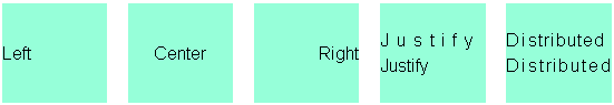
Horizontal alignment
Set the alignment mode of data in a cell in the horizontal direction – “Left”, “Center”, “Right”, “Justify” and “Distributed”。
● Example:
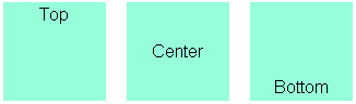
Vertical alignment
Set the alignment mode of data in a cell in the horizontal direction – “Top”, “Center” and “Bottom”.
● Example:
Indent
Set the indentation of the data value in a cell. Default indent value is 0, which positions the value close to the border. Generally, the indentation is set as 2-3.
★ Note:
1.After the “Indent” property is configured, text will be indented a certain distance from the left/right margin or both. If the horizontal alignment mode is “Left”, text will be indented from the left margin; if it is “Center”, text will be indented from both the left and right margins; if it is “Right”, text will be indented from the right margin.
2.It is recommended that the “Indent” property not be configured for a statistical graph, that is, make the indentation 0 – because once the image is compressed, it becomes deformed and affect the outcome.
3.It is recommended that the “Indent” property not be configured for an intersection cell in a crosstab.
● Example: As the following shows, indentation from the left is 0 and that from the right is 5.
![]()
Font
This section illustrates font size, bold, italic, underline properties of general cells.
Font Name
Set font for a value/display value in a cell.
★ Note:
If the server has a non-Windows OS, such as Linux and Unix, you need to install all fonts that will be possibly used in OS. Without installing them, the report will be shown as gibberish or small squares when being print as or export to PDF, or has its statistical graphs exported. Generally, install corresponding installation package first and then JDK. If the JDK is already installed, you can copy the fonts to the OS.
Method of coping the fonts is this: Copy all font files in …\WINDOWS\Fonts directory under Windows to the server’s JDK installation directory’s subdirectory …\jre\lib\fonts. If this is useless for certain operation systems, you may need to open …\jre\lib\font.properties file and make some modifications.
Font Size
Set font size for a value/display value in a cell.
● Example: As the following shows, the left is 12pt and the right is 22pt.
![]()
Bold
Choose whether to show data in a cell as bold.
● Example: As the following shows, the left is the effect when “Bold” property isn’t configured and the right is the effect after it is selected.
![]()
Italic
Choose whether to display data in a cell in italic.
● Example: As the following shows, the left is the effect when “Italic” property isn’t configured and the right is the effect after it is selected.
![]()
Underline
Choose whether to underline data in a cell.
● Example: As the following shows, the left is the effect of showing data without an underline and the right is the effect of underlining the data.
![]()
Expansion
A function whose computing result is a set is called a set function. Such functions include group(), select(), list(), query() and to().
Take to() function as an example, like to(1,3).
An expression whose computing result is a set is called a set expression.
An expression whose computing result is a single value is called a single-value expression.
When the data value expression for a cell is a set expression, this cell is by default an expanding cell; otherwise the cell is considered as non-expanding.
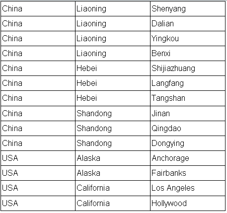
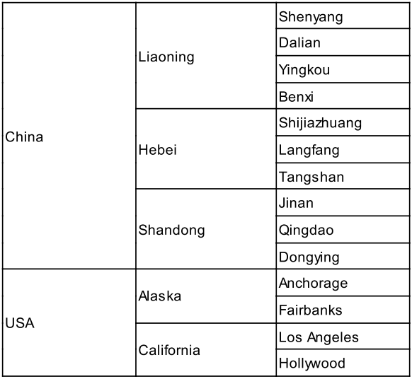
Expanding Mode
There are four types of expanding mode for a cell – “Default”, “Horizontal”, “Vertical” and “None”. For an expanding cell, its expansion direction can be default or you can set an expansion direction for it. The cell can expand in two directions, that is, horizontal expansion and vertical expansion. But one expanding cell cannot expand in two directions at the same time.
1. Default
l When expression for a cell is a single-value expression, this cell is by default non-expandable;
l When expression for a cell is a set expression, this cell is by default expandable;
l When an expanding cell’s master cell is the row primary cell or column primary cell, the cell is by default vertically expandable;
l When an expanding cell’s top master cell is horizontally expandable, the cell is by default horizontally expandable;
l When an expanding cell’s left master cell is vertically expandable, the cell is by default vertically expandable;
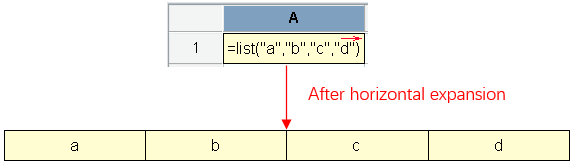
2. Horizontal
l When the expansion direction of an expanding cell is horizontal, the cell’s expansion is a horizontal expansion, which enables the cell to be copied horizontally. Values of the result duplicate cells are results of the expression in order. The number of cells the cell expands to is the number of values the expression returns;
l All properties of the new cells reference properties of the cell from which they are copied.
Example:
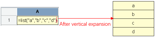
3. Vertical
l When the expansion direction of an expanding cell is vertical, the cell’s expansion is a vertical expansion, which enables the cell to be copied vertically. Values of the result duplicate cells are results of the expression in order. The number of cells the cell expands to is the number of values the expression returns;
l All properties of the new cells reference properties of the cell from which they are copied.
Example:
4. None
l When value of the expression in a cell is a single value, the cell is by default non-expandable.
Left Master Cell
For a vertically expanding cell, it is the left master cell of the cell to the right. The “Left Master Cell” property is by default absent or can be modified.
Default identification rule for left master cell:
For a vertically expanding cell, the vertically expanding cell directly to the left is by default its left master cell, and the cell directly to the right is by default its subordinate cell; if there isn’t a such a cell on the left, its left master cell is by default cell `0.
The specified left master cell setting rule:
You can set a cell’s left master cell as a vertically expanding cell. If you need to change the cell’s left master cell to 00 cell, just configure the “Left master cell” property value as `0.
To conform to the expansion rules, we need to set the left master cell according to the following rules:
Ø A left master cell should be vertically expanding, otherwise the setting is invalid;
Ø A circular setting is not permitted, such as setting A’s left master cell as B, B’s left master cell as C and C’s left master cell as A, and is regarded as an error that makes report computations unable to proceed. Such a setting is impossible by default, but it should be avoided under the specified setting;
Ø A horizontally expanding cell cannot have a left master cell.
During a specified setting, it is possible that a cell’s left master cell is to its right and it is not necessarily that the left master cell and its subordinate cell are in the same row.
Top Master Cell
A horizontally expanding cell is the top master cell of the cell directly below it.
Default identification rule for top master cell:
For a horizontally expanding cell, the horizontally expanding cell directly above it is by default its top master cell, and the cell directly below it is by default its subordinate cell; if there isn’t a such a cell above it, its top master cell is by default cell `0.
The specified top master cell setting rule:
You can set a cell’s top master cell as a horizontally expanding cell. If you need to change the cell’s top master cell to 00 cell, just configure the “Top master cell” property value as `0.
To conform to the expansion rules, we need to set the top master cell according to the following rules:
Ø A top master cell should be horizontally expanding, otherwise the setting is invalid;
Ø A circular setting is not permitted, such as setting A’s top master cell as B, B’s top master cell as C and C’s top master cell as A, and is regarded as an error that makes report computations unable to proceed. Such a setting is impossible by default, but it should be avoided under the specified setting;
Ø A vertically expanding cell cannot have a top master cell.
During a specified setting, it is possible that a cell’s top master cell is below it and it is not necessarily that the top master cell and its subordinate cell are in the same column.
Merge Same value
For a report where page breaks are set up, you can set the merge mode for adjacent cells having same values after expansion. There are four merge modes – No merge, Horizontal merge, Vertical merge, and Bidirectional merge. The same value merge is valid only for cells expanded from the same expanding master cell.
1. When selecting “No merge”, adjacent cells having same values won’t be merged into a single bigger cell.
● Example: “No merge” is set for A1 and B1.
Below is the effect of printing or exporting a certain page:
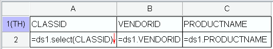
2. By selecting “Horizontal merge”, adjacent cells having same values in the horizontal direction will be merged horizontally into a bigger cell. The merge order is top-down by row.
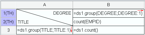
● Example: Set “Horizontal merge” for A1 and A2.
Below is the effect of printing or exporting a certain page:

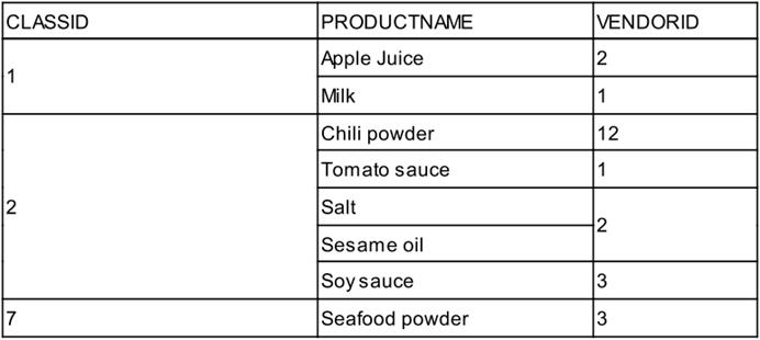
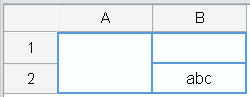
Generally, a cell in one column contains certain other cells or is contained by a certain cell. Cells in this same column won’t intersect. So, same value merge won’t happen if intersection will be incurred, for instance:
In the above screenshot, cells having same value in the blue box cannot be merged because their merge will cause intersection with the cell highlighted in red.
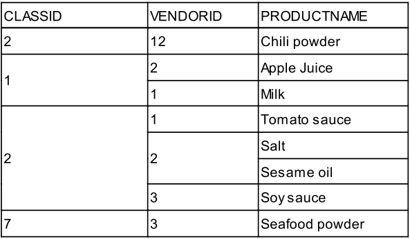
3. When “Vertical merge” is selected, adjacent cells having same values in the vertical direction will be merged vertically into a bigger cell. The merge order is from left to right by column.
● Example: Set “Vertical merge” for A1 and A2.
Below is the effect of printing or exporting a certain page:
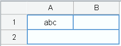
Generally, a cell in one row contains certain other cells or is contained by a certain cell. Cells in this same row won’t intersect. So, same value merge won’t happen if intersection will be incurred, for instance:
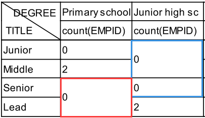
In the above screenshot, cells having same value in the blue box cannot be merged because their merge will cause intersection with the cell highlighted in red.
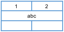
4. When “Bidirectional merge” is chosen, adjacent cells having same values in both directions will be merged into a bigger cell. The property applies to the crosstab. The merge order is vertical (from left to right by column) and then horizontal (from top to bottom).
● Example: “Bidirectional merge” is set for B3.
Below is the effect of printing or exporting a certain page:
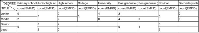
According to the above screenshot, a cell in one row/column contains certain other cells or is contained by a certain cell. Cells in this same row/column won’t intersect. So, same value merge won’t happen if intersection will be incurred.
Note:
“Merge Same Value” is valid only when page breaks are configured. When no page breaks are set or a paginated report is export to a non-paginated Excel/PDF file, the property becomes invalid.
Same Value Merge Style
When page breaks are set for a report, you can set a style for cells on which same value merge will be performed. There are four styles – Default, Normal, Reverse, and Simple. The most common merge style is “Default”.
1. With “Default” style, only cells having same master cell will be merged.
● Example: “Vertical merge” merge mode and “Default” same value merge style are set for C2.
Below is the preview effect:
2. When the same value merge style is “Simple”, adjacent cells having same value will be merged even they are not under the same master cell.
● Example: “Vertical merge” merge mode and “Simple” same value merge style are set for C2.
Below is the effect of printing or exporting a certain page:

3. Set same value merge style as “Normal” and the merge will be performed in the order of left to right and top-down.
● Example: “Vertical merge” merge mode is set for A2 and B2, “Normal” same value merge style is set for A2, and “Default” same value merge style is set for B2.
Below is the effect of printing or exporting a certain page:
4. Set same value merge style as “Reverse” and the merge will be performed in the order of bottom-up and right to left.
● Example: “Vertical merge” merge mode is set for A2 and B2, “Reverse” same value merge style is set for A2, and “Default” same value merge style is set for B2.
Below is the effect of printing or exporting a certain page:
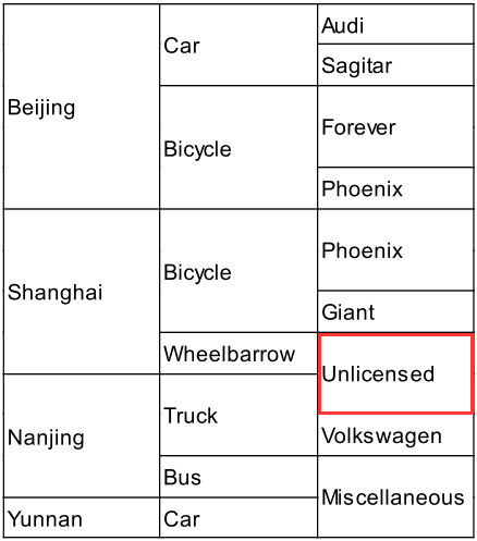
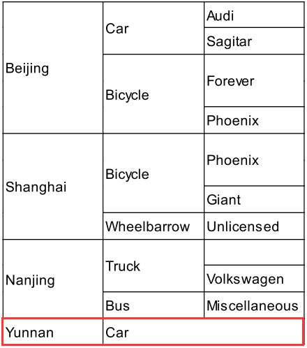
Merge Null Value
For a report where page breaks are set up, you can set the merge mode for cells containing null values after expansion. There are five merge modes – No merge, Merge up, Merge down, Merge left, and Merge right.
A null-value cell to be merged can come from a different expanding master cell.
To merge null-value cells bottom-up/top-down, cells in the vertical direction must be have same width.
To merge null-value cells leftward/rightward, cells in the horizontal direction must be have same height.
You can set different null-value merge mode for different null-value cells. Perform merge across the whole table in one direction and then in the other direction. The merge order is top-down, bottom-up, leftward and rightward.
When both same value merge and null value merge are set for a report, perform the former first and then the latter.
1. When “No merge” is selected, a null-value cell won’t be merged with its neighboring cell.
● Example: Set “No merge” for C1.
Below is the preview effect:
2. When “Merge up”/“Merge down” is selected, a null-value cell will merge with the neighboring cell above/below it in the same column and having same width.
● Example: Set “Merge up” for C1.
When a null-value cell gets a neibouring, same-width cell in the same column to merge with it, you get the following effect of printing or exporting a certain report page:
3. When “Merge left”/“Merge right” is selected, a null-value cell will merge with the neighboring cell to the left/right in the same row and having same height.
● Example: Set “Merge left” for C1.
When a null-value cell gets a neibouring, same-height cell in the same row to merge with it, you get the following effect of printing or exporting a certain report page:
4. Different null-value cells can have different merge mode. Perform merge across the whole table in one direction and then in the other direction. The merge order is top-down, bottom-up, leftward and rightward.
● Example: Set “Merge right” for A1 and “Merge down” for B1.
Perform top-down merge and then rightward merge. Below is the result:

● Example: Set “Merge left” for B1 and “Merge up” for A2.
Perform bottom-up merge and then leftward merge. As there isn’t a same-width cell directly above A2, you get the following result:

5. Perform Merge Same Value and then Merge Null Value.
● Example: Set Merge Same Value -> Horizontal merge for A2 and Merge Null Value -> Merge up for A3.
Perform same-value merge first. As there isn’t a same-width cell directly above A3 for null-value merge, you get the following result:
Note:
“Merge Null Value” is valid only when page breaks are configured. When no page breaks are set or a paginated report is export to a non-paginated Excel/PDF file, the property becomes invalid.
Hyperlink
The “Hyperlink” property of a cell can be a “Value” or an “Expression”.
If a hyperlink string does not need to be generated dynamically, you can just write the path to be linked under the property’s “Value”.
If the hyperlink string needs to be dynamically generated according to the cell or parameter value, write the path to be linked under the property’s “Expression”.
URL Target
Hyperlink jump method:
1. When the property value is _self, jump to a location within the current page.
2. When the property value is _blank, jump to a new page.
When this property is left empty, use default value _self.
Page Break
This section illustrates page break, clustered-column report and cell unmerge.
Stretch At Page Break
The property applies to all areas except for report header, group header, data area and report footer.
Page Break After Row
Choose whether to break page after the current row. The property can be a value or an expression.
The property enables page breaks forcefully. You can set page break according to the number of data rows and by specifying the number of rows displayed per page. Sometimes you may just want to define page break after a certain row or certain rows, rather than showing a fixed number of rows in each page. This property lets you achieve that.
It can be set for a general cell or a row primary cell.
By setting it for the row primary cell and the corresponding row is expandable, the property will be copied to all cells expanded from this row.
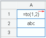
● Example:
Edit =to(1,10) in A1, and enter expression if(A1= =5,true,false) for the cell’s “Page Break After Row” property. According to the expression, when value of the current cell is 5, page breaks after the row. A preview after print shows that the row containing value 6 is displayed in the next page.
Page Break After Column
Choose whether to break page after the current column. The property can be a value or an expression. Choose whether to break page after the current row. It can be set for a general cell or a column primary cell. The configuration rule is same as that for “Page Break After Row”.
Clustered Columns After Row
Choose whether to create clustered columns after a specified row. The property can be a value or an expression.
Sometimes you may just want to define clustered columns after a certain row or certain rows, rather than showing a fixed number of rows in each page. This property lets you achieve that.
It can be set for a general cell or a row primary cell.
By setting it for the row primary cell and the corresponding row is expandable, the property will be copied to all cells expanded from this row.
● Example:
Edit =to(1,10) in A1, and enter expression if(A1= =5,true,false) for the cell’s “Clustered Columns After Row” property. According to the expression, when value of the current cell is 5, create clustered columns after the row. A preview after print shows that the row containing value 6 is displayed in clustered columns.
Unmerge cell
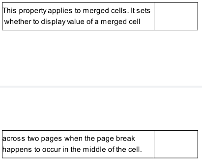
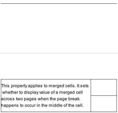
This property applies to merged cells. It sets whether to display value of a merged cell across two pages when the page break happens to occur in the middle of the cell.
● Example: As the following shows:
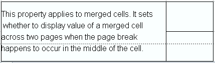
The page break occurs in the middle of the merged cell.
By configuring this property, text in this merged cell will be split into two parts and displayed across two pages, as the following shows:
When this property is not set, text in this merged cell is displayed on the second page.
Other
This section illustrates a series of properties, including comment on general cells, export-to-Excel style, Editable or not, cell style and editable/non-editable expressions.
Note
You can make notes and comments about cells in a report through “Note” property for the convenience of others’ viewing or yourself looking up later.
Export-to-Excel Style
You can control whether to display default values, real values, display values or formulas when exporting the report to an Excel file through this property.
Export Default Value: Using this style, the export result is consistent with the preview effect.
Real Value: Using this style, the export result displays “Value + Display Format”.
Display Value: Using this style, the export result displays “Display Value + Display Format”.
Formula: When the cell value expression is a formula Excel can identify, export it as a formula; when it isn’t, simply export the computing result.
Formulas Excel can identify include the basic arithmetic operations (like A1+A2), aggregate functions (such as sum, avg, max and min), simple mathematical and trigonometric functions (such as abs, exp, lg, ln, sin, cos, tan, asin, acos and atan), and certain commonly used string functions (such as left, right, len, upper and lower).
● Example:
Example 1: Get GENDER value from A1. The original value in A1 is “F” or “M”. Set display value expression as map(list("F","M"),list("Female","Male")) for A1, and:
For preview: Display “Male” or “Female”;
When exporting Real Value: Display “M” or “F”;
When exporting Display Value: Display “Male” or “Female”.
Example 2: Get SALARY value from A1. One of the original values is “7,000”. Set display value expression as “ds1.SALARY+1000” for A1 and display format as “¥#.00”.
For preview: Display “¥8000.00”;
When exporting Real Value: Display “¥7000.00”;
When exporting Display Value: Display “¥8000.00”.
Example 3: In A2, compute sum of SALARY values in the cells expanded from A1. Set value expession as =sum(A1{}) for A2 and display format as “¥#.00”.
For preview: Display “¥18000.00”;
When exporting Formula: Display “=SUM(A1:A2)”, and its value is “¥18000.00”.
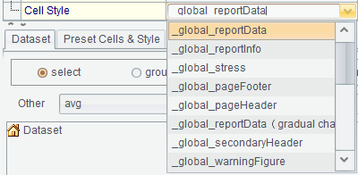
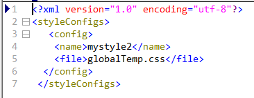
Cell Style
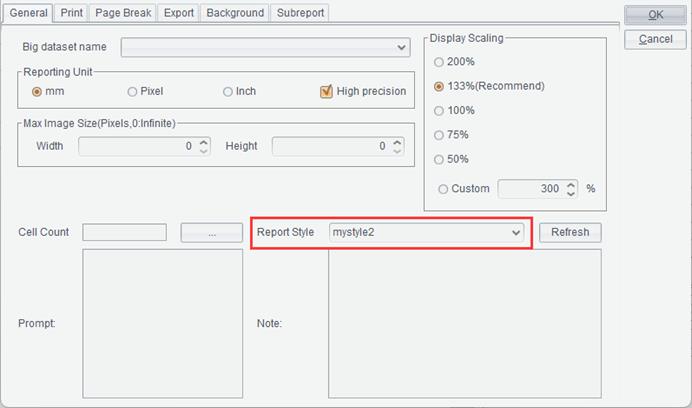
Set style of a cell. Read cell style list from the .css file pointed by the report style configured in Report -> Report properties. Read report properties’ report styles from the report style .xml file configured in File tab in Tools -> Options.
After report style is set in report properties, this style will be automatically listed in the report style list in the Property area on the right part of the designer. Below are the configurations:
reportStyleConfig.xml:
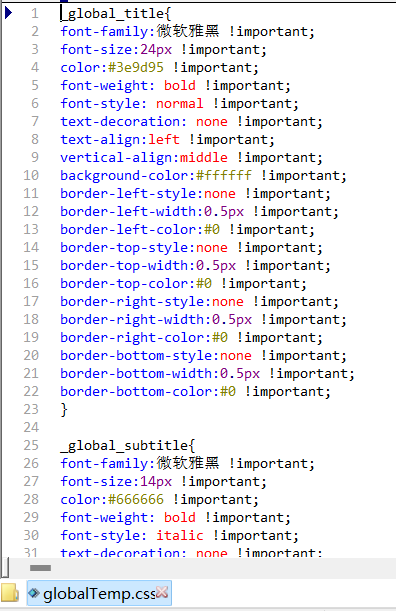
globalTemp.css: