Math
1. The directory containing files of this external library is: installation directory\esProc\extlib\MathCli. The Raqsoft core jar for this external library is scu-math-cli-2.10.jar.
ejml-core-0.40.jar
ejml-ddense-0.40.jar
ejml-simple-0.40.jar
libsvm-3.25.jar
Note: The third-party jars are encapsulated in the compression package and users can choose appropriate ones for specific scenarios.
2. esProc provides functions chi2inv(), cov(), covm() and dism() to access the Math external library. Look them up in【Help】-【Function reference】to find their uses.
3. The MathCli external library provides certain linear algebra-related functions. They have the following uses:
(1) Generate a matrix
In MathCli, we can use functions to generate a zero matrix, unit matrix, etc. For example:
|
|
A |
B |
|
1 |
=I(3) |
|
|
2 |
=eye(3) |
=eye(4, 3) |
|
3 |
=ones(3) |
=ones(4, 3) |
|
4 |
=zeros(3) |
=zeros(4, 3) |
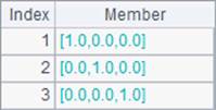
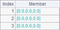
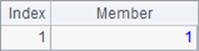
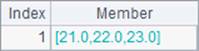
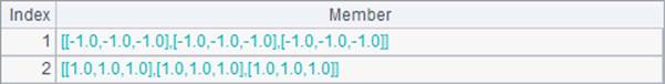
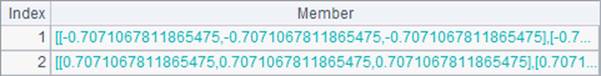
Both I() function and eye() function can be used to generate a unit matrix. A unit matrix is a matrix where the main diagonal element is equal to 1 and the remaining elements are 0. Different of the two functions are that I() function can only define a square matrix. Results of A1, A2 and B2 in the above cellset code are as follows:

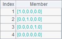
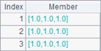
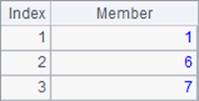
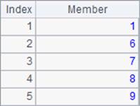
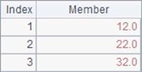
Similar to eye() function, ones() function and zeros() function can generate a matrix of ones and a zero matrix. But different from eye() function, they can also define a multidimensional matrix through using parameters. Results A3`B4 are as follows:


(2) Perform operations on multidimensional matrices
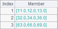
We can use mfind(A, n) function to find positions of the first n non-zero members in vector or matrix A. For example:
|
|
A |
B |
|
1 |
[0,,3,2,0,2,1,0] |
=mfind(A1) |
|
2 |
=mfind(A1,3) |
=mfind(A1,10) |
|
3 |
[[1,0,2],[0,0,2],[0,4,7]] |
=mfind(A3) |
|
4 |
=mfind(A3,3) |
=mfind(A3,10) |
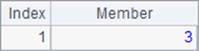
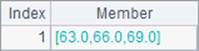
When A is a vector, the function returns an array consisting of ordinal numbers of the non-zero members in the vector; the ordinal number starts from 1. When parameter n is absent, the function only returns the position of the first non-zero member, as B1 does. The result is as follows:
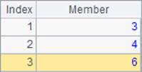
When parameter n is present, the function returns positions of the first n non-zero members. When the number of all non-zero members is less than n, the function returns positions of all non-zero members. Below are results of A2 and B2:
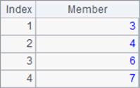
When A is a matrix, the function returns an array consisting of ordinal numbers of the non-zero members in the matrix; the search begins from the first columns. For example, in the matrix defined in line 3 in the above cellset code, positions of the first columns are 1, 2 and 3 respectively, and those of the second columns are 4, 5 and 6 respectively, and so on. When parameter n is absent, the function only returns the position of the first non-zero, non-null member, as B3 does. Its result is as follows:
When parameter n is present, the function returns positions of the first n non-zero members. When the number of all non-zero members is less than n, the function returns positions of all non-zero, non-null members. Below are results of A4 and B4:
In the external library MathCli, msum(A, n) function is used to perform a sum aggregation operation on an ordinary matrix or a multidimensional matrix. In the function, parameter n is the number of dimension levels. For example:
|
|
A |
B |
|
1 |
[[11,12,13],[21,22,23],[31,32,33]] |
=msum@a(A1) |
|
2 |
=msum(A1, 1) |
=msum(A1, 2) |
|
3 |
[[[111,112,113],[121,122,123],[131,132,133]],[[211,212,213],[221,222,223],[231,232,233]]] |
=msum@a(A3) |
|
4 |
=msum(A3, 1) |
=msum(A3, 2) |
A1 defines an ordinary matrix:
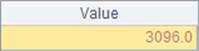
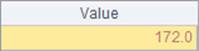
When working with @a option, msum function calculates sum of all members of the matrix. Here’s result of B1:
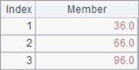
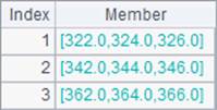
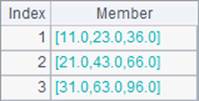
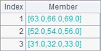
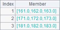
We can specify the number of dimension levels for the aggregation through parameter n. When n is absent, the function summarizes values on the first level only. When there is only one member on the first level, summarize values on the second level; and so on. With a matrix, aggregation on the first level means summing values of rows respectively and that on the second level means summing values of columns respectively. Below are results of A2 and B2:
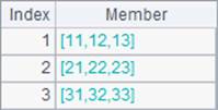
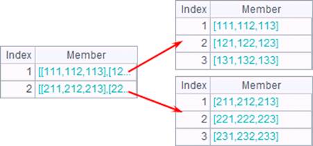
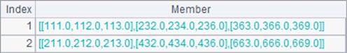
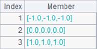
A3 defines a three-dimensional matrix (as shown below). Two of its members are a 3*3 matrix:
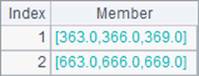
With the @a option, msum function also calculates the sum of all members in the multi-dimensional matrix. Here’s result of B3:
We can specify the number of dimension levels for the sum through parameter n. When n is absent, the function summarizes values on the first level only. With a multidimensional matrix, sum on the first level means performing alignment addition on the above two matrices, and sum on the second level means getting sum of members of each column in each of the two matrices respectively. Below are results of A4 and B4:
In MathCli external library function, we can also use mcumsum(A, n) function to calculate the cumulative sum on an ordinary matrix or a multidimensional matrix. For example:
|
|
A |
B |
|
1 |
[[11,12,13],[21,22,23],[31,32,33]] |
=mcumsum(A1) |
|
2 |
=mcumsum(A1, 2) |
=mcumsum@z(A1) |
|
3 |
[[[111,112,113],[121,122,123],[131,132,133]],[[211,212,213],[221,222,223],[231,232,233]]] |
|
|
4 |
=mcumsum(A3) |
=mcumsum(A3, 2) |
The mcumsum function returns the cumulative sum, which is different from the result of an ordinary sum operation. B1 and A2 calculate the cumulative sum on each row and on each column respectively. Their results are as follows:
We can use @z option with mcumsum function to get the cumulative sum in the inverse order, as B2 does. Its result is as follows:
We can also specify the number of dimension levels for the cumulative sum operation on a multidimensional matrix. If we do not specify it, just perform cumulative sum operation on the first level. Below are results of A4 and B4:

The mmean(A, n) function is used to calculate the mean value on an ordinary matrix or a multidimensional matrix. For example:
|
|
A |
B |
|
1 |
[[11,12,13],[21,22,23],[31,32,33]] |
=mmean@a(A1) |
|
2 |
=mmean(A1) |
=mmean(A1, 2) |
|
3 |
[[[111,112,113],[121,122,123],[131,132,133]],[[211,212,213],[221,222,223],[231,232,233]]] |
=mmean@a(A3) |
|
4 |
=mmean(A3) |
=mmean(A3, 2) |
Similar to calculating the sum, the mmean function calculates the mean value of all members of the matrix when working with @a option. Here’s result of B1:
As we do with the sum operation, we can specify the number of dimension levels in the mmean function. A2 and B2 calculate the mean value of each column and that of each column respectively. Results are as follows:
When calculating the mean value on a multidimensional matrix, the mmean function can also add @a option to calculate the mean value of all members of the matrix, as B3 does. Here’s its result:
The number of dimension levels can also be specified for the calculation of mean value on a multidimensional matrix. Below are results of A4 and B4:
The MathClic external library offers mtd(A, n) function to calculate the standard deviation on an ordinary matrix or a multidimensional matrix. For example:
|
|
A |
B |
|
1 |
[[11,12,13],[21,22,23],[31,32,33]] |
=mstd(A1) |
|
2 |
=mstd(A1, 2) |
=mstd@s(A1) |
|
3 |
[[[111,112,113],[121,122,123],[131,132,133]],[[211,212,213],[221,222,223],[231,232,233]]] |
=mstd(A3) |
|
4 |
=mstd(A3, 2) |
=mstd@s(A3) |
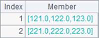
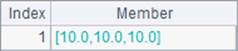
We can specify the number of dimension levels in the mstd function for calculating the standard deviation. B1 and A2 respectively calculates the standard deviation of each column and that of each row in the matrix. Their results are as follows:
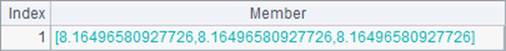
The mstd function can add an @s option to use a statistical algorithm to calculate the standard deviation. The algorithm uses n-1to find the mean value. Below is result of B2:
Calculating the standard deviation on a multidimensional matrix is similar to getting sum on it. Results of B3 and A4 are as follows:
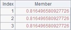
B4 uses the @s option and gets the following result:
In the mnorm(A, n) function, we can specify the dimension, and normalize data in an ordinary matrix or a multidimensional matrix to make the mean value of members on the specified dimension levels 0 and standard deviation 1. For example:
|
|
A |
B |
|
1 |
[[11,12,13],[21,22,23],[31,32,33]] |
=mnorm(A1) |
|
2 |
=mnorm(A1, 2) |
=mnorm@s(A1) |
|
3 |
[[[111,112,113],[121,122,123],[131,132,133]],[[211,212,213],[221,222,223],[231,232,233]]] |
=mnorm(A3) |
|
4 |
=mnorm(A3, 2) |
=mnorm@s(A3) |
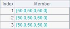
The mnorm function has similar uses to uses of previous functions. B1 and A2 respectively normalize data in each column and data in each column in the matrix. Here are their results:
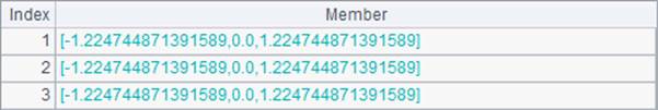
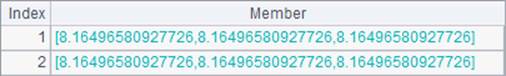
With the @s option, the mnorm function uses a statistical algorithm to find standard deviation during normalization, as B2 does. Here’s its result:
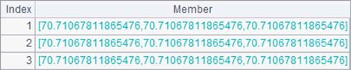
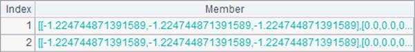
Like calculating sum, calculating the standard deviation on a multidimensional matrix uses the same way. Here are results of B3 and B4:
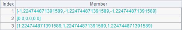
B4 adds @s option and get the following result:
(3) Offer inverse cumulative distribution functions
The MathCli external library supplies inverse cumulative distribution functions. For example:
|
|
A |
|
1 |
=norminv(0.25, 2, 1) |
|
2 |
=tinv(0.99, 2) |
|
3 |
=finv(0.95,5,10) |
|
4 |
=chi2inv(0.95,10) |
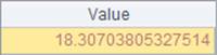
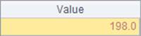
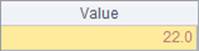
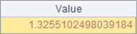
The norminv(p, mu, sigma) function calculates normal inverse cumulative distribution, in which probability p is within the interval (0, 1), parameter mu is the specified mean value, and parameter sigma is the specified standard deviation. Here’s result of A1:
The tinv(p, nu) function calculates the inverse T cumulative distribution, in which probability p is within the interval (0, 1) and parameter nu is the degrees of freedom corresponding to the probability. A2’s result is as follows:
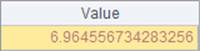
The finv(p, v1, v2) function calculates the inverse F cumulative distribution, in which probability p is within the interval (0, 1), parameter v1 is the numerator degrees of freedom, and parameter v2 is the denominator degrees of freedom. Here’s result of A3:
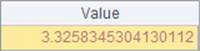
The chi2inv(p, v) function calculates the chi-square inverse cumulative distribution, in which probability p is within the interval (0, 1) and parameter v is the degrees of freedom. Here’s result of A4: