Cluster computations

esProc allows using cluster computing to perform complicated analytic and processing tasks. A cluster system consists of multiple clustered servers running on a network of independent computers. Every single computer in the network can send a cluster computing request to the cluster.

A cluster system enhances computational performance significantly by gathering the computational power of multiple servers. It can be expanded whenever necessary without paying the high cost associated with the mainframe.

10.3.1 Performing cluster computations with callx function

We learned how to launch the parallel servers in The Server Cluster. After clustered servers are started and a cluster system is created, cluster computation can be performed through callx function. In esProc, every server will carry out the cluster computing tasks by computing the specified script file and returning the result.

To perform a cluster computation, first prepare the cellset file to be calculated by the subtasks, like CalcStock.splx shown below:

	A	B
1	>output@t("calc begin, SID="+string(arg1) +". ")	=file("StockRecord.txt").cursor@t()
2	=B1.select(SID==arg1)	=A2.fetch()
3	=B2.count()	=B2.max(Closing)
4	=B2.min(Closing)	=round(B2.avg(Closing),2)
5	>output@t("calc finish, SID="+string(arg1) +". ")	return A3,B3,A4,B4

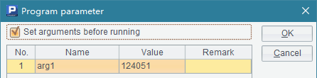
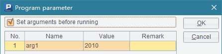
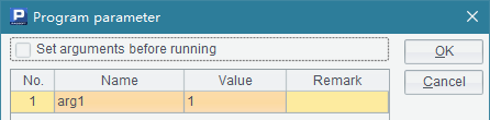
The StockRecord.txt file contains closing prices of some stocks in a certain period of time. Each subtask computes the transaction information for stocks of specified codes, including the total number of trading days, the highest and lowest closing prices and the average closing price. The average closing price will be simply computed by trading days, without taking the number of transactions into consideration. In order to know the detailed information about the execution of subtasks, output@t function is used at the beginning of the computation and before result returning to output the times and prompts. In the cellset file, arg1 is a parameter for passing stock codes in and needs to be set before the cluster computation. Select Set arguments before running to set the parameter:

Cluster computing requires that in computers that run clustered servers the cellset file CalcStock.splx should exist and be placed in the mainPath or the search path configured for every server.

This computation involves one node A, whose IP address is 192.168.1.112:8281 and on which the maximum number of tasks allowed is three.

Then you can start the cluster computation using callx function in the esProc main program on any computer in the network:

	A
1	[192.168.1.112:8281]
2	[124051,128857,131893,136760,139951,145380]
3	=callx("CalcStock.splx",A2;A1)
4	=A3.new(A2(#):SID,~(1):Count,~(2):Maximum,~(3):Minimum,~(4):Average)

About callx’s parameters in A3’s expression, the two before the semicolon are used for computing the cellset file. The cluster computing will divide the computational task into multiple subtasks according to the sequence parameter; the length of the sequence parameter is the number of subtasks. As with here, the multiple parameters are separated by the comma, in which a single-value parameter, if any, will be duplicated to every subtask. The parameter after the semicolon is the sequence of nodes, each of which is represented by its IP and port number, which is a string in the format of “IP:port number”, like “192.168.1.112:8281” used in the current example. After the computation on a clustered server is completed, the result set needs to be returned by the return statement; multiple result sets will be returned in the form of a sequence.

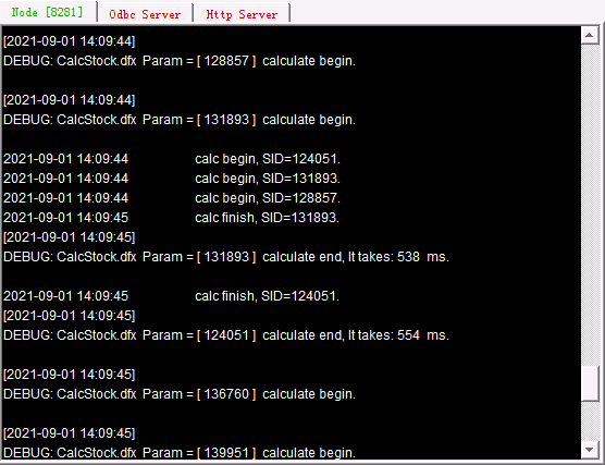
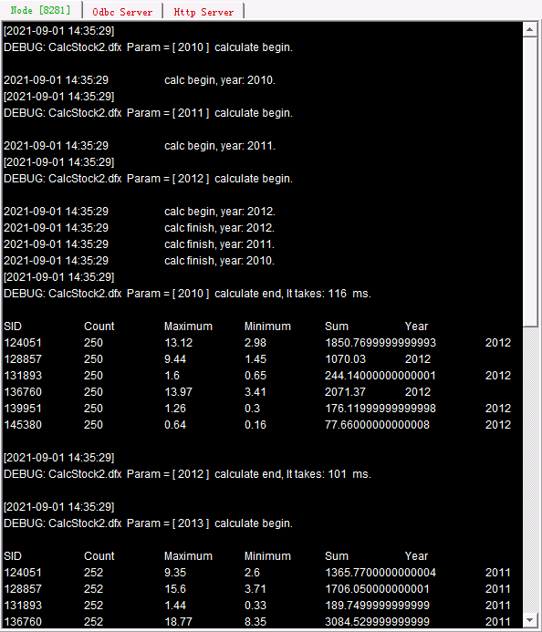
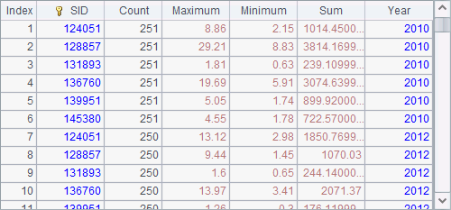
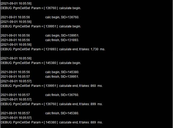
In this example, data of six stocks are computed. Their codes are 124051,128857,131893,136760,139951,145380, which correspond tasks a, b, c, d, e, f that will be distributed among nodes during the cluster computation. When there are multiple nodes in the node list, tasks will be allocated to them in turn. When the number of tasks being performed on every node reaches the limit, task assignment will be suspended until there is a finished task. If a node isn’t started or the number of processes running on it reaches its maximum, then move on to the next node in the list. We can read the distribution and execution messages of tasks on each of their System Output window. There is only one node in use in this example, and below is the related information:

(Continued)

 

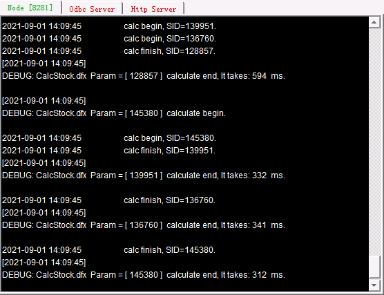
As can be seen from the output information, Tasks a, b, c are first allocated and executed, and the remainng tasks d, e, f are waiting in queue for a sequential allocation until there is an available process.

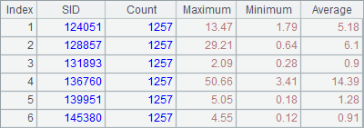
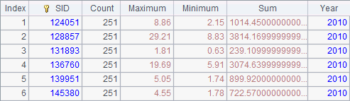
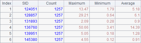
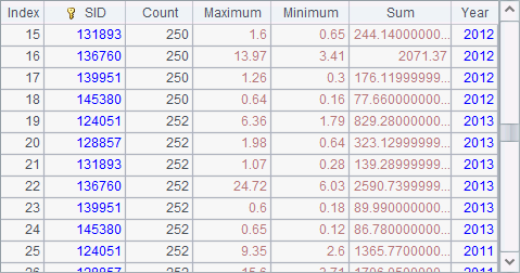
After the computations are completed, the result can be viewed in A4:

This example shows that, by splitting apart a data-intensive computational task and having each process handle one of the parts, cluster computing can make full use of the computers’ computing ability to increase efficiency and effectively avoid the memory overflow usually happened during big data processing by using multiple computers to run nodes.

As tasks are executed separately on each node, they are independent of each other. And the data source and the data file needed in the computation on a node should be already configured and stored on it. So, the script file must be placed on each node beforehand. You can also use callx@a to allocate tasks randomly.

Let’s look at another example. Still, we’ll get the statistical data of the six stocks, but this time each process only gets data of a certain year. The corresponding cellset file CalcStock2.splx is as follows:

	A	B
1	>output@t("calc begin, year: "+string(arg1)+". ")	=file("StockRecord"+string(arg1)+".txt")
2	=B1.cursor@t()	[124051,128857,131893,136760,139951,145380]
3	=A2.select(B3.pos(SID)>0).fetch()	=A3.groups(SID;count(~):Count,max(Closing):Maximum,min(Closing):Minimum,sum(Closing):Sum)
4	>output@t("calc finish, year: "+string(arg1)+". ")	return B3.derive(arg1:Year)

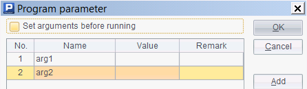
Stock data of different years are stored in their respective data files. For example, the data of 2010 is stored in StockRecord2010.txt. The five data files used for computation are from 2010 to 2014. Each task computes the transaction data of the six stocks in a specified year. As in the above example, output@t function is used to output times and prompts as the computation begins and before the result is returned.

In the cellset file, arg1 is a parameter that passes a specified year whose data is to be computed and that is added in B4’s return result for checking:

Then perform cluster computation in the main program:

	A
1	[192.168.1.112:8281]
2	[2010,2011,2012,2013,2014]
3	=callx("CalcStock2.splx",A2;A1; "reduce_addRecord.splx")
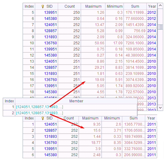
4	=A3.conj().group(SID;~.max(Maximum):Maximum,~.min(Minimum):Minimum,round(~.sum(Sum)/~.sum(Count),2):Averge)

A3 performs cluster computation using callx(spl,…;h:rspl) function. The function has a reduce script file rspl. Below is the reduce script:

	A
1	return arg1|arg2

arg1 and arg2 are parameters defined for the script file:

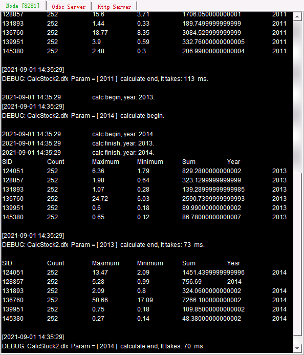
Here we do not need to assign values to the parameters and care about their names. They will be respectively assigned with the current cumulative result of executing reduce and the result returned from the current task. The script unions records returned by all tasks. Each task executes reduce to get a new cumulative value ~~ after it returns its own result. After callx is executed, status of the task distribution and execution is displayed on each server’s System Output window:

(Continueed)

 

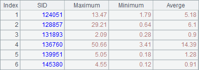
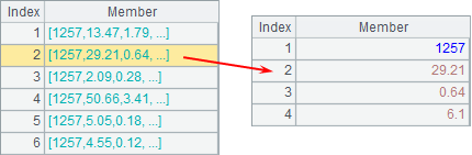
A3’s result is a sequence, whose members are as follows:

By executing reduce actions, callx gets a record sequence of result records returned from tasks.

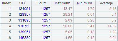
A4 concatenates the returned results and groups and aggregates A3’s result to calculate the highest and lowest prices and the average price:

 

During a cluster computation involving multiple nodes, if there are nodes that can’t handle the tasks allocated to it, the task distribution is problematic. The disuse of option in callx function will strictly distribute each task to the server storing the correponding data file. In this case the number of subtask should be same as the number of nodes.

Now we add a Node II 192.168.1.112:8282 Node II stores three data files – StockRecord2010.txt, StockRecord2011.txt and StockRecord2012.txt in its main path. We use the following program to perform cluster computation over the above stock data:

	A
1	[192.168.1.112:8281,192.168.1.112:8282]
2	[2010,2011,2012,2013,2014]
3	=callx("CalcStock2.splx",A2;A1; "reduce_addRecord.splx")
4	=A3.conj().group(SID;~.max(Maximum):Maximum,~.min(Minimum):Minimum,round(~.sum(Sum)/~.sum(Count),2):Averge)

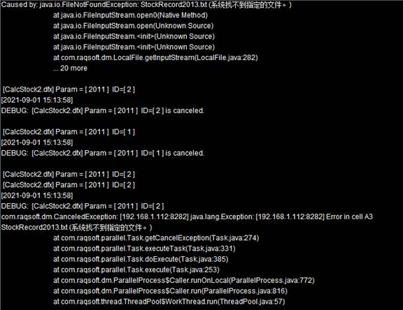
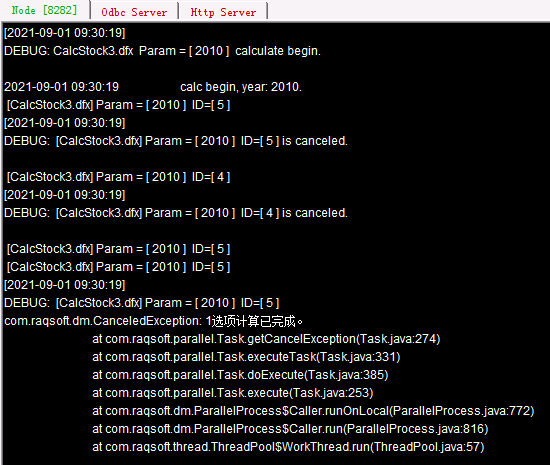
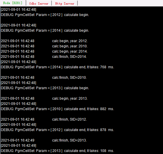
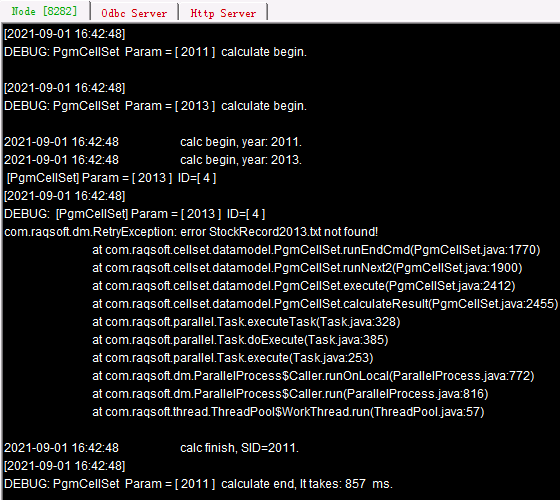
In this example, a cluster system consisting of multiple nodes is used. The main node assigns tasks to the nodes in turn. Specifically speaking, task 2010 is given to node Ⅰ, task 2011 is given to node II , and in turn, task 2012 is allocated to node Ⅰ and task 2013 is for node II. Yet, as Node II doesn’t have all the data files needed to get the tasks done, the execution reports error:

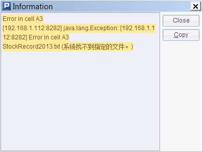
We can view error details in the Node Server information output windows for the nodes:

 

In order to avoid the error, we edit the script executed in callx function to add an end statement before a probable computing error, which signifies an abnormal termination and enables a reassignment by the cluster system. To edit CalcStock2.splx and save it as CalcStock3.splx, for instance:

	A	B
1	>output@t("calc begin, year: "+string(arg1)+". ")	=file("StockRecord"+string(arg1)+".txt")
2	if !B1.exists()	end B1.name()+" not found!"
3	=B1.cursor@t()	[124051,128857,131893,136760,139951,145380]
4	=A3.select(B3.pos(SID)>0).fetch()	=A4.groups(SID;count(~):Count,max(Closing):Maximum, min(Closing):Minimum,sum(Closing):Sum)
5	>output@t("calc finish, year: "+string(arg1)+". ")	return B4.derive(arg1:Year)

Row 2 is the newly-added. If B1’s file does not exist, the end statement returns the information of abnormal termination saying that the file does not exist.

	A
1	[192.168.1.112:8281,192.168.1.112:8282]
2	[2010,2011,2012,2013,2014]
3	=callx("CalcStock3.splx",A2;A1; "reduce_addRecord.splx")
4	=A3.conj().group(SID;~.max(Maximum):Maximum,~.min(Minimum):Minimum, round(~.sum(Sum)/~.sum(Count),2):Averge)

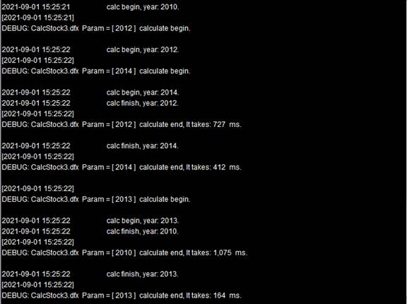
Now the execution will goes on normally.View how the tasks are distributed by clicking cell A3:

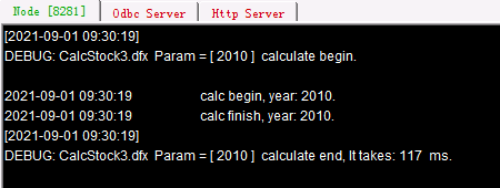
Task assignment will be still in order. It gives task 2010, task 2012 and task 2014 to node Ⅰ, and task 2011 and task 2013 to node Ⅱ. When node Ⅱ cannot find the corresponding file when trying to handle task 2013, it executes end statement to return the related information and enables a reassignment of the task to node Ⅰ, making the computation completed successfully. Below is the system information output from the two nodes:

 

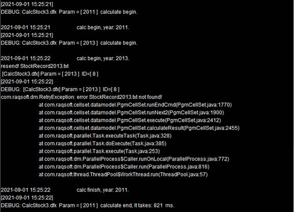
 According to the information, task 2013 is sent back to the system for reallocation after it fails on node Ⅱ. It happens that node Ⅰ has finished performing a task and can receive one more task. So, task 2013 is given to it. Note that here A4 will first union the results returned from the two nodes before performing the aggregation. Here’s A3’s result:

The records in the result are the same as those obtained from the single node computation.

As we can see from the above instance, there may be potential troubles when certain tasks can only be performed on a certain node, and the end statement is needed to manage the abnormal termination.Otherwise, it may trigger the failure of the whole task if one of the servers goes wrong. To avoid the previously-happened issue that not all nodes have all the necessary files, we use callx to execute a script that calls syncfile(hs, p) function to synchronize all files in path p on node list hs across the nodes, during which an old file will be replaced by the namesake new one.

 

On certain occasions, we can perform one task on multiple nodes, for instance:

	A
1	[192.168.1.112:8281,192.168.1.112:8282]
2	[2010]
3	=callx@1("CalcStock3.splx",A2;A1)
4	=A3.conj()

Here only stock data of the year 2010 is computed. The corresponding file is stored on both nodes. call() function uses @1 option to give the single task to both nodes. One node will stop its task execution as long as the other completes handling the task. Here is information displayed on the clustered server information output windows:

As you can see, node Ⅱ exits the task execution after node Ⅰ completes the task. Below is A4’ result:

@1 option can be used to perform a task similar to random searches on multiple nodes and the task is successfully completed as long as one node finishes handling it.

 

10.3.2 Performing cluster computations with fork statement

Multithreading discussed that the fork statement can be used to execute a piece of code using multiple theads. The callx() function used in the above section is responsible for executing a script file at each of the servers in cluster.

So callx’s work can be done by fork statement. For example:

	A	B	C
1	[192.168.11.112:8281]
2	[124051,128857,131893,136760,139951,145380]
3	fork A2;A1	>output@t("calc begin, SID="+string(A3) +". ")
4		=file("StockRecord.txt").import@t()	=B4.select(SID==A3)
5		=C4.count()	=C4.max(Closing)
6		=C4.min(Closing)	=round(C4.avg(Closing),2)
7		>output@t("calc finish, SID="+string(A3) +". ")	return B5,C5,B6,C6
8	=A3.new(A2(#):SID,~(1):Count,~(2):Maximum,~(3):Minimum,~(4):Average)

This is functionally equivalent to writing a subroutine requiring repeated execution in a code block, saving the effort of maintaining multiple script files. During a cluster computation, add task number sequence s at the end of the fork statement to distribute tasks to certain nodes, like fork A2;A1:[[4,5],[1,2,3]]. A3 collects results of all tasks and return the following:

The order of the records returned by A3 is in line with the parameter order. A8 further processes the result of the cluster computations and return the following table:

The computation uses one node, whose execution informatin can be viewed on the Node Server system output window:

 

We can also add reduce actions in the fork statement:

	A	B	C
1	[192.168.1.112:8281]
2	[124051,128857,131893,136760,139951,145380]
3	fork A2;A1	>output@t("calc begin, SID="+string(A3) +". ")
4		=file("StockRecord.txt").import@t()	=B4.select(SID==A3)
5		=C4.count()	=C4.max(Closing)
6		=C4.min(Closing)	=round(C4.avg(Closing),2)
7		>output@t("calc finish, SID="+string(A3) +". ")	return A3,B5,C5,B6,C6
8	reduce	=if(ift(A3),A3.record(A8),create(SID, Count, Maximum, Minimum, Average ).record(A3).record(A8))
9	=A3.conj()

The reduce code block uses reduce functions. It creates the result table sequence when performing the first reduce and populate the first task result in A3 that stores the current cumulative value and the current second task result returned by A8 to the newly-created table sequence. The subsequent reduce actions will add their returned records to the table sequence accordingly. A3’s value changes from fork code block to reduce code block. The cell receives the parameter value in the former and stores the cumulative value in the latter. Here’s the result of the cluster computation in A3 after execution:

As only one node is involved, the table sequence it returns is the final aggregate result.

The fork statement can also perform tasks using multiple nodes, for instance:

	A	B	C
1	[192.168.1.112:8281, 192.168.1.112:8282]
2	[2010,2011,2012,2013,2014]	[124051,128857,131893,136760,139951,145380]
3	fork A2;A1	>output@t("calc begin, year: "+string(A3)+". ")	=file("StockRecord"/A3/".txt")
4		if !C3.exists()	end C3.name()+" not found!"
5		=C3.cursor@t()
6		=B5.select(B2.pos(SID)>0).fetch()	=B6.groups(SID;count(~):Count,max(Closing):Maximum, min(Closing):Minimum,sum(Closing):Sum)
7		>output@t("calc finish, SID="+string(A3) +". ")	result C6.derive(A3:Year)
8	reduce	=A3|A8
9	=A3.conj().

In the above cellset file, fork statement is used to compute data of specified stocks in all years. In the code block, line 4 checks whether the necessary file exists and uses end statement to return abnormal termination information and enable a reassignment of the task if the file cannot be found on the current node. Line 8 uses reduce statement to concatenate result records returned by all nodes. Similar to the example in the previous section where the end statement is added to reduce script, a task that cannot be computed by a node will be redistributed during execution. Here is output information of two nodes:

Task 2013 is given to node Ⅱ according to the default assignment order and then reallocated to node Ⅰ when the former terminates the computation abnormally. Make a note that both reduce statement and reduce script performs a cumulative operation only on a single node when doing a reduce action. The execution order is related to the task execution efficiency and assignment order. So, in the result returned by A9, we can see that the order of records is consistent with that of nodes and task assignment:

Usually, the result will be sorted again. If the reduce statement isn’t used, the result will have a same order with the parameters.

10.3.3 Handling computation-intensive tasks

In the previous examples, cluster computing is used to handle data-intensive computational tasks. By processing part of the data in each process, it makes the most use of the limited memory. In other scenarios, the task involves extremely complicated computation that can also be split apart through cluster computing into multiple subtasks that will be distributed among multiple nodes for execution. Results of the subtasks will be merged by the main node.

Take the following subroutine CalcPi.splx as an example:

	A	B	C
1	1000000	0	>output@t("Task "+ string(arg1)+ " start...")
2	for A1	=rand()	=rand()
3		=B2*B2+C2*C2
4		if B3<1	>B1=B1+1
5	>output@t("Task "+ string(arg1)+ " finish.")	return B1

Parameter arg1 is used to record serial numbers of subtasks:

This subroutine is created to estimate the value of π - ratio of circumference to diameter - using probability theory. Look at the following picture:

There is the quarter-circle in a square with side length of 1. The area of the square is 1 and the area of the sector is π/4. The probability of a point of the square that falls in the sector is the ratio of their areas, i.e.π/4. This subroutine randomly generates 1,000,000 points whose x, y coordinates are within the interval [0,1), computes the distance of each of these points from the origin, records the number of points that fall in the sector and then estimates the value of π.

Here’s the main program:

	A	B
1	[192.168.1.112:8281, 192.168.1.112:8281, 192.168.1.112:8283]	20
2	CalcPi.splx	=movefile@cy(A2;"/", A1)
2	=callx(A2, to(B1);A1)	=A3.sum()*4/(1000000d*B1)

Start node Ⅲ first and its main path is D:/files/node3. The above code, before calling the node, first copies the necessary script file onto all nodes using movefile() function that uses @c option and @y option to disable deletion of the source file and enable overwriting a namesake file. By invoking the subroutine 20 times, the cluster computing distributes the computations of 20,000,000 points among processes (they are those used in the previous section). Distribution and execution information of the tasks can be viewed on each clustered server’s System Output window:

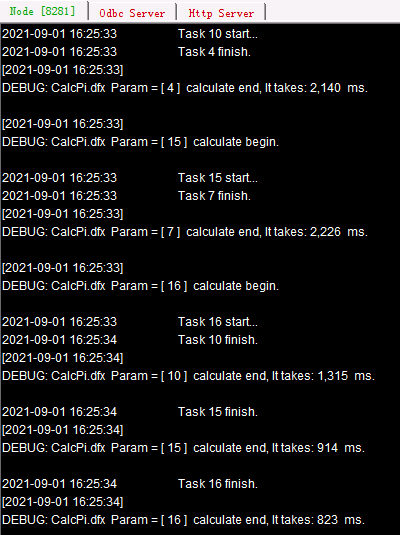
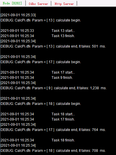
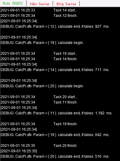
If the number of tasks exceeds the maximum task number the nodes can handle and processes on all nodes have already received their tasks, the subsequent tasks need to wait to be distributed until a process is available. In this case a task will be given to any idle process, so distribution solutions may vary. Each task computation process is independent. A task distributed later than another one may be accomplished earlier, which will not affect the final result of cluster computing.

The approximate value of π is computed in B2. Because the computation is performed based on probability, results are slightly different from each other.